latent code (잠재 벡터)차원이 줄어든채로 데이터를 잘 설명할 수 있는 잠재 공간에서의 벡터
latent code == latent vector == latent space
loss
학습된 모델에 실제 데이터를 입력으로 주었을 때 모델의 추정 오차로 발생하는 손실.
실제 정답과 학습된 모델이 예측한 값 사이 차이(거리, 오차)
손실이 클수록
loss 함수
파라미터에 대한 evaluation(cost)
모델이 예측한 값과 실제 정답 사이 차이 비교하는 함수
loss
GAN (Generative Adversarial Network)Generator(진짜 같은 이미지 생성하려는 생성 모델)와 Discriminator의 경쟁을 통해 학습(적대적 학습)하여 Generator에서 실제 이미지와 구분이 되지 않는 거짓 이미지를 생성
Minmax problem
G: Generator, D: DiscriminatorD(x) : Discriminator → 진짜일 확률이 0 ~ 1 사이 값이라 데이터가 진짜면 D(x)=1, 가짜면 D(x)=0⇒ 분류자 D의 maxV(D,G)의 의미: V(D,G)가 최대가 되도록 D를 학습한다는 판별자가 진짜 데이터를 진짜로, 가짜 데이터를 가짜로 분류하도록 학습하는 것으로 logD(x)와 log(1-D(G(z)))가 최대이어야 함. 즉, D(x)는 실제 데이터를 진짜로 분류하도록 D를 학습하는 것이고, 1-D(G(z)) 최대이려면 D(G(z))는 최소이어야 하므로 D(G(z))=0이 되도록, G(생성자)가 만들어낸 가짜 데이터를 가짜로 분류하도록 D를 학습해야 함
⇒ 생성자 G의 minV(D,G)의 의미: V(D,G)가 최소가 되도록 학습하는 것. 첫 번째 항은 G가 포함되어 있지 않으므로 생략. 두 번째 항에서 최소가 되려면 log(1-D(G(z)))에서 1-D(G(z))이 최소가 되어야 하고, 따라서 D(G(z))=1이어야 함. 즉, G가 생성한 가짜 데이터를 D에서 진짜로 분류하도록 학습해야 함.
D(G(z)) : G가 만든 데이터 G(z)를 분류자에 넣어서 진짜로 판단 시 D(G(z))=1, 가짜로 판단 시 D(G(z))=0
z: latent vector → 차원이 줄어든채로 데이터를 잘 설명할 수 있는 잠재 공간에서의 벡터
GAN에는 진짜 같은 데이터를 생성하려는 생성 모델과 진짜와 가짜를 판별하려는 분류 모델이 존재하여 서로 적대적으로 학습하여 서로 경쟁적으로 발전하는 구조. 적대적 학습에서 먼저 분류 모델을 학습하고, 학습된 분류 모델을 속이도록 생성 모델을 학습하여 서로 주고받으면서 반복됨.
Generator와 Discriminator로 구성된 딥러닝 모델
GAN의 구성
Generator
Discriminator
노이즈(z)를 입력받아 latent code로부터 실제 이미지와 유사한 샘플(ex. 이미지) 생성
평가(생성 분포가 훈련 분포와 구별 가능 여부를 판별하는 함수) 수행하기 위해 discriminator network 훈련
Generator가 학습되면 폐기되는 adaptive loss 함수(적응 손실 함수)
진짜 데이터 분류모델에 입력받아서 네트워크가 해당 데이터를 진짜로 분류하도록 학습시키는 과정
생성 모델에서 생성한 가짜 데이터를 분류모델에 입력받아서 해당 데이터를 가짜로 분류하도록 학습시키는 과정
Generator 생성 모델의 학습→ 생성 모델이 생성한 가짜 데이터를 분류 모델에서 진짜로 분류하도록 분류 모델을 속이는 것이 목표
생성 모델에서 생성한 가짜 데이터를 판별 모델에 입력으로 넣어서 가짜 데이터를 진짜로 분류하도록 진짜와 유사한 데이터를 생성하도록 학습
Discriminator 분류 모델의 학습→ 진짜 데이터를 진짜로, 가짜 데이터를 가짜로 분류하는 것이 목표
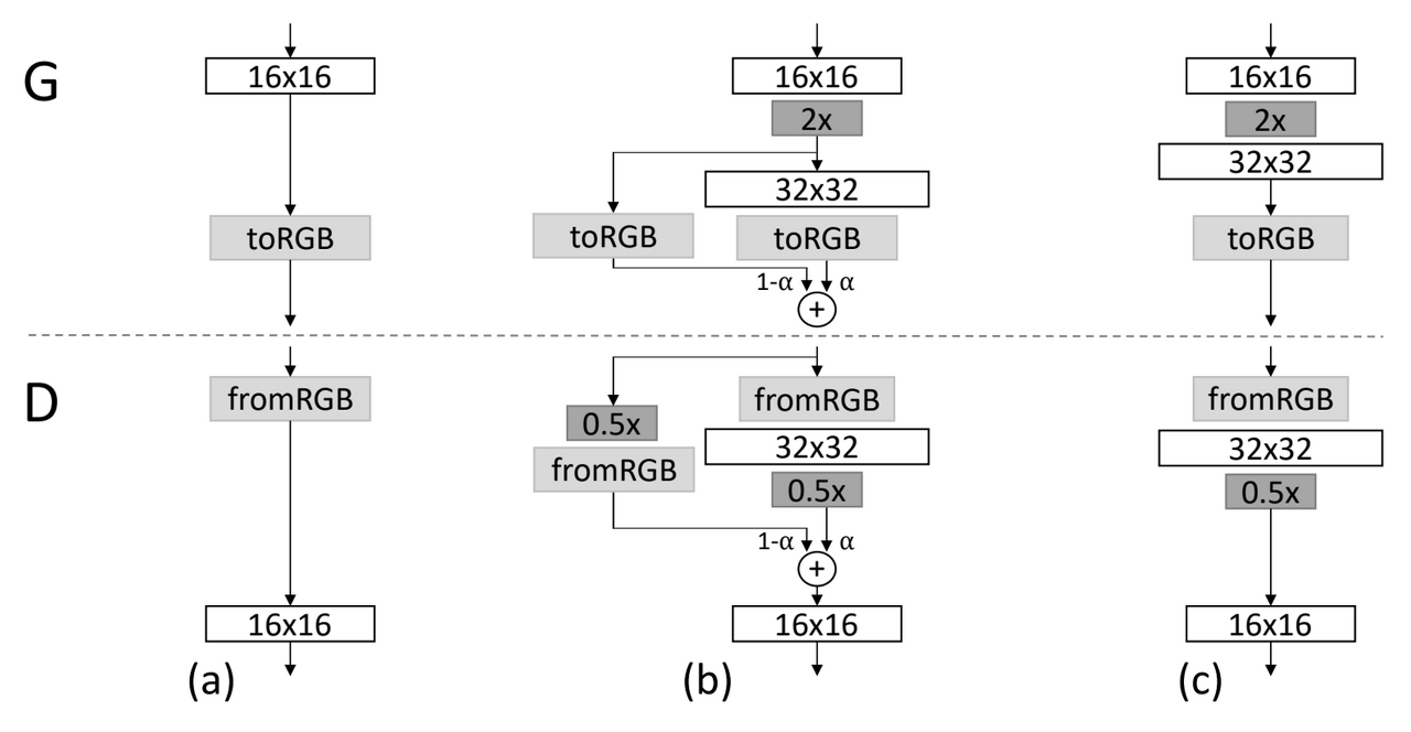
Generator: α를 처음에는 0으로 초기화(16 x 16을 2x(근사 이웃 필터링과 평균 풀링을 사용하여 해상도를 2배로 늘림)로 upsampling하여 toRGB layer를 거치게 함)하고, 새로운 layer가 완전히 공간에 들어올 때까지 점차 α를 0부터 1까지 선형적으로 증가시키면서 학습. 해상도를 32 x 32까지 높이면서 학습 시 기존에 학습한 이미지 정보(16 x 16)을 잃을 수 있으므로 residual block을 이용하여 한 번 더 학습을 안정화
Discriminator: discriminator 훈련 시 네트워크의 현재 해상도에 맞게 축소된 실제 이미지를 입력해야 한다. 따라서 generator의 출력 이미지 32 x 32를 discriminator에서 사용하기 위해 보간을 수행하여 해상도를 전환한다. 이때 0.5x는 이미지 해상도를 절반으로 줄이는 것을 의미.
(c) stabilize
discriminator에서 해상도를 줄일 때에도 학습 안정성을 위해 fade in 해준다.
progressive training 장점
stability
저해상도 이미지에는 더 적은 class 정보와 mode가 있기 때문에 저해상도 이미지부터 생성하는 것이 더 안정적
reduced training time
2~6배 더 빠르게 결과를 얻을 수 있음
2. minibatch standard deviation : mode collapse 해결
minibatch discrimination (Salimans et al. 2016)
GAN의 mode collapse(훈련 데이터에서 발견되는 변이의 일부만 포착하는 경향)을 해결하기 위해 제안됨
minibatch 전체에서 feature statistics를 계산하여 생성된 이미지와 학습 이미지의 minibatch가 유사한 통계를 보이도록 유도→ discriminator가 이 통계 정보를 활용하여 거짓의 생성된 batch로부터 진짜 학습 데이터 batch를 구별하는데 도움이 됨
minibatch layer
통계 배열에 입력 activation을 투영하는 큰 tensor를 학습한다. minibatch에서 각 샘플에 대한 통계 배열이 생성되고, minibatch layer의 출력에 연결되어 discriminator에서 해당 통계를 내부적으로 사용할 수 있다.
PGGAN에서의 minibatch standard deviation
minibatch discrimination 접근 방식을 간소화하고 변이 개선
학습 가능한 매개변수, hyperparameter 없음
minibatch에서 각 공간 위치의 특징에 대한 표준편차 계산→ 해당 단일값을 복제하고 단일값을 모든 공간 위치와 minibatch에 연결하여 하나의 추가 feature map을 생성함
→ 모든 특징과 공간 위치의 추정치에 대한 평균을 구하여 단일값에 도달
구현 방법: discriminator 끝에 4 x 4 해상도에 추가 feature map으로써 across-minibatch 표준 편차 추가 (minibatch layer 추가)
→ 이유: discriminator 끝에 minibatch layer 추가하는게 가장 좋았는데, 그 이유는 (appendix A.1)
3. equalized learning rate & Pixelwise normalization : GAN에서 신호 크기와 경쟁 제한
generator에서 3 x 3 convolution layer 후 feature vector에 대해 pixelwise normalization 적용
일반적으로 사용되는 adaptive stochastic gradient descent 방법은 기울기 업데이트를 추정 표준편차로 정규화하여 매개변수의 규모와 무관하게 업데이트가 되어 일부 파라미터의 동적 범위가 다른 파라미터보다 큰 경우 조정하는데 시간이 오래 걸림
equalized learning rate는 모든 가중치에 대해 동적 범위, 즉 학습 속도가 동일함을 보장함
(2) pixelwise feature vector normalization (G와 D의 경쟁 제한, 신호 크기 증폭 제한)
local response normalization
ax,y bx,y : 각 픽셀(x,y)의 원본 및 정규화된 feature vector N: # of feature maps
목적: generator와 discriminator에서 경쟁으로 인해 generator와 discriminator의 크기가 통제 불가능 상태가 되는 상황 방지
각 pixel의 feature vector를 convolutional layer한 후 generator의 단위 길이에 맞게 정규화한다.
local response normalization 변형 사용
신호 크기(signal magnitude)가 증폭되는 것을 효과적으로 방지 가능
signal magnitude
입력 신호의 크기로, 학습 데이터와 생성된 데이터의 신호 크기 비교하여 모델 성능 평가
4. Multi-scale statistical similarity : GAN 결과 평가
한 GAN의 결과를 다른 GAN과 비교하기 위해 대규모 이미지 컬렉션에서 지표를 계산하는 자동화된 방법 사용
기존 MS-SSIM 방법 한계: 대규모 mode collapse는 안정적으로 찾지만 색상이나 질감에서의 다양성 손실과 같은 작은 영향에 대처를 못함
⇒ 좋은 generator는 모든 scale에 대해 학습 set과 로컬 이미지 구조가 비슷하다는 multi-scale statistical similarity 사용 제안
Implementation
Generator와 Discriminator 구조
훈련에 사용한 데이터셋
CELEBA-HQ dataset
훈련 방법
4 x 4 해상도부터 시작해서 discriminator에서 800만 개의 실제 이미지를 보여줄 때까지 네트워크 훈련하고, 다음 800만 개 이미지에 대해서는 첫 번째 3-layer 블록을 fade in하고 800만 개 이미지에 대한 네트워크를 안정화 한 후 800만 개 대상으로 다음 3-layer 블록을 fade in하는 과정을 반복함.
latent vector
512차원 hypersphere에서의 임의의 점
훈련 및 생성 이미지를 [-1, 1]로 표현
activation 함수
G, D의 마지막 layer: linear activation
이를 제외한 모든 layer: leakiness가 0.2인 leaky ReLU(Rectified Linear Unit) 사용
normalization
generator에서 각 3 x 3 convolution layer 후의 feature vector에 pixelwise normalization 적용
# Minibatch standard deviation.

def minibatch_stddev_layer(x, group_size=4):
    with tf.variable_scope('MinibatchStddev'):
        group_size = tf.minimum(group_size, tf.shape(x)[0])     # Minibatch must be divisible by (or smaller than) group_size.
        s = x.shape                                             # [NCHW]  Input shape.
        y = tf.reshape(x, [group_size, -1, s[1], s[2], s[3]])   # [GMCHW] Split minibatch into M groups of size G.
        y = tf.cast(y, tf.float32)                              # [GMCHW] Cast to FP32.
        y -= tf.reduce_mean(y, axis=0, keepdims=True)           # [GMCHW] Subtract mean over group.
        y = tf.reduce_mean(tf.square(y), axis=0)                # [MCHW]  Calc variance over group.
        y = tf.sqrt(y + 1e-8)                                   # [MCHW]  Calc stddev over group.
        y = tf.reduce_mean(y, axis=[1,2,3], keepdims=True)      # [M111]  Take average over fmaps and pixels.
        y = tf.cast(y, x.dtype)                                 # [M111]  Cast back to original data type.
        y = tf.tile(y, [group_size, 1, s[2], s[3]])             # [N1HW]  Replicate over group and pixels.
        return tf.concat([x, y], axis=1)                        # [NCHW]  Append as new fmap.
pixelwise feature vector normalization
# Pixelwise feature vector normalization.

def pixel_norm(x, epsilon=1e-8):
    with tf.variable_scope('PixelNorm'):
        return x * tf.rsqrt(tf.reduce_mean(tf.square(x), axis=1, keepdims=True) + epsilon)
Generator
논문에 사용된 generator 코드
# Generator network used in the paper.

def G_paper(
    latents_in,                         # First input: Latent vectors [minibatch, latent_size].
    labels_in,                          # Second input: Labels [minibatch, label_size].
    num_channels        = 1,            # Number of output color channels. Overridden based on dataset.
    resolution          = 32,           # Output resolution. Overridden based on dataset.
    label_size          = 0,            # Dimensionality of the labels, 0 if no labels. Overridden based on dataset.
    fmap_base           = 8192,         # Overall multiplier for the number of feature maps.
    fmap_decay          = 1.0,          # log2 feature map reduction when doubling the resolution.
    fmap_max            = 512,          # Maximum number of feature maps in any layer.
    latent_size         = None,         # Dimensionality of the latent vectors. None = min(fmap_base, fmap_max).
    normalize_latents   = True,         # Normalize latent vectors before feeding them to the network?
    use_wscale          = True,         # Enable equalized learning rate?
    use_pixelnorm       = True,         # Enable pixelwise feature vector normalization?
    pixelnorm_epsilon   = 1e-8,         # Constant epsilon for pixelwise feature vector normalization.
    use_leakyrelu       = True,         # True = leaky ReLU, False = ReLU.
    dtype               = 'float32',    # Data type to use for activations and outputs.
    fused_scale         = True,         # True = use fused upscale2d + conv2d, False = separate upscale2d layers.
    structure           = None,         # 'linear' = human-readable, 'recursive' = efficient, None = select automatically.
    is_template_graph   = False,        # True = template graph constructed by the Network class, False = actual evaluation.
    **kwargs):                          # Ignore unrecognized keyword args.

    resolution_log2 = int(np.log2(resolution))
    assert resolution == 2**resolution_log2 and resolution >= 4
    def nf(stage): return min(int(fmap_base / (2.0 ** (stage * fmap_decay))), fmap_max)
    def PN(x): return pixel_norm(x, epsilon=pixelnorm_epsilon) if use_pixelnorm else x
    if latent_size is None: latent_size = nf(0)
    if structure is None: structure = 'linear' if is_template_graph else 'recursive'
    act = leaky_relu if use_leakyrelu else tf.nn.relu

    latents_in.set_shape([None, latent_size])
    labels_in.set_shape([None, label_size])
    combo_in = tf.cast(tf.concat([latents_in, labels_in], axis=1), dtype)
    lod_in = tf.cast(tf.get_variable('lod', initializer=np.float32(0.0), trainable=False), dtype)

    # Building blocks.
    def block(x, res): # res = 2..resolution_log2
        with tf.variable_scope('%dx%d' % (2**res, 2**res)):
            if res == 2: # 4x4
                if normalize_latents: x = pixel_norm(x, epsilon=pixelnorm_epsilon)
                with tf.variable_scope('Dense'):
                    x = dense(x, fmaps=nf(res-1)*16, gain=np.sqrt(2)/4, use_wscale=use_wscale) # override gain to match the original Theano implementation
                    x = tf.reshape(x, [-1, nf(res-1), 4, 4])
                    x = PN(act(apply_bias(x)))
                with tf.variable_scope('Conv'):
                    x = PN(act(apply_bias(conv2d(x, fmaps=nf(res-1), kernel=3, use_wscale=use_wscale))))
            else: # 8x8 and up
                if fused_scale:
                    with tf.variable_scope('Conv0_up'):
                        x = PN(act(apply_bias(upscale2d_conv2d(x, fmaps=nf(res-1), kernel=3, use_wscale=use_wscale))))
                else:
                    x = upscale2d(x)
                    with tf.variable_scope('Conv0'):
                        x = PN(act(apply_bias(conv2d(x, fmaps=nf(res-1), kernel=3, use_wscale=use_wscale))))
                with tf.variable_scope('Conv1'):
                    x = PN(act(apply_bias(conv2d(x, fmaps=nf(res-1), kernel=3, use_wscale=use_wscale))))
            return x
    def torgb(x, res): # res = 2..resolution_log2
        lod = resolution_log2 - res
        with tf.variable_scope('ToRGB_lod%d' % lod):
            return apply_bias(conv2d(x, fmaps=num_channels, kernel=1, gain=1, use_wscale=use_wscale))

    # Linear structure: simple but inefficient.
    if structure == 'linear':
        x = block(combo_in, 2)
        images_out = torgb(x, 2)
        for res in range(3, resolution_log2 + 1):
            lod = resolution_log2 - res
            x = block(x, res)
            img = torgb(x, res)
            images_out = upscale2d(images_out)
            with tf.variable_scope('Grow_lod%d' % lod):
                images_out = lerp_clip(img, images_out, lod_in - lod)

    # Recursive structure: complex but efficient.
    if structure == 'recursive':
        def grow(x, res, lod):
            y = block(x, res)
            img = lambda: upscale2d(torgb(y, res), 2**lod)
            if res > 2: img = cset(img, (lod_in > lod), lambda: upscale2d(lerp(torgb(y, res), upscale2d(torgb(x, res - 1)), lod_in - lod), 2**lod))
            if lod > 0: img = cset(img, (lod_in < lod), lambda: grow(y, res + 1, lod - 1))
            return img()
        images_out = grow(combo_in, 2, resolution_log2 - 2)

    assert images_out.dtype == tf.as_dtype(dtype)
    images_out = tf.identity(images_out, name='images_out')
    return
Discriminator
논문에 사용된 Discriminator 코드
# Discriminator network used in the paper.

def D_paper(
    images_in,                          # Input: Images [minibatch, channel, height, width].
    num_channels        = 1,            # Number of input color channels. Overridden based on dataset.
    resolution          = 32,           # Input resolution. Overridden based on dataset.
    label_size          = 0,            # Dimensionality of the labels, 0 if no labels. Overridden based on dataset.
    fmap_base           = 8192,         # Overall multiplier for the number of feature maps.
    fmap_decay          = 1.0,          # log2 feature map reduction when doubling the resolution.
    fmap_max            = 512,          # Maximum number of feature maps in any layer.
    use_wscale          = True,         # Enable equalized learning rate?
    mbstd_group_size    = 4,            # Group size for the minibatch standard deviation layer, 0 = disable.
    dtype               = 'float32',    # Data type to use for activations and outputs.
    fused_scale         = True,         # True = use fused conv2d + downscale2d, False = separate downscale2d layers.
    structure           = None,         # 'linear' = human-readable, 'recursive' = efficient, None = select automatically
    is_template_graph   = False,        # True = template graph constructed by the Network class, False = actual evaluation.
    **kwargs):                          # Ignore unrecognized keyword args.

    resolution_log2 = int(np.log2(resolution))
    assert resolution == 2**resolution_log2 and resolution >= 4
    def nf(stage): return min(int(fmap_base / (2.0 ** (stage * fmap_decay))), fmap_max)
    if structure is None: structure = 'linear' if is_template_graph else 'recursive'
    act = leaky_relu

    images_in.set_shape([None, num_channels, resolution, resolution])
    images_in = tf.cast(images_in, dtype)
    lod_in = tf.cast(tf.get_variable('lod', initializer=np.float32(0.0), trainable=False), dtype)

    # Building blocks.
    def fromrgb(x, res): # res = 2..resolution_log2
        with tf.variable_scope('FromRGB_lod%d' % (resolution_log2 - res)):
            return act(apply_bias(conv2d(x, fmaps=nf(res-1), kernel=1, use_wscale=use_wscale)))
    def block(x, res): # res = 2..resolution_log2
        with tf.variable_scope('%dx%d' % (2**res, 2**res)):
            if res >= 3: # 8x8 and up
                with tf.variable_scope('Conv0'):
                    x = act(apply_bias(conv2d(x, fmaps=nf(res-1), kernel=3, use_wscale=use_wscale)))
                if fused_scale:
                    with tf.variable_scope('Conv1_down'):
                        x = act(apply_bias(conv2d_downscale2d(x, fmaps=nf(res-2), kernel=3, use_wscale=use_wscale)))
                else:
                    with tf.variable_scope('Conv1'):
                        x = act(apply_bias(conv2d(x, fmaps=nf(res-2), kernel=3, use_wscale=use_wscale)))
                    x = downscale2d(x)
            else: # 4x4
                if mbstd_group_size > 1:
                    x = minibatch_stddev_layer(x, mbstd_group_size)
                with tf.variable_scope('Conv'):
                    x = act(apply_bias(conv2d(x, fmaps=nf(res-1), kernel=3, use_wscale=use_wscale)))
                with tf.variable_scope('Dense0'):
                    x = act(apply_bias(dense(x, fmaps=nf(res-2), use_wscale=use_wscale)))
                with tf.variable_scope('Dense1'):
                    x = apply_bias(dense(x, fmaps=1+label_size, gain=1, use_wscale=use_wscale))
            return x

    # Linear structure: simple but inefficient.
    if structure == 'linear':
        img = images_in
        x = fromrgb(img, resolution_log2)
        for res in range(resolution_log2, 2, -1):
            lod = resolution_log2 - res
            x = block(x, res)
            img = downscale2d(img)
            y = fromrgb(img, res - 1)
            with tf.variable_scope('Grow_lod%d' % lod):
                x = lerp_clip(x, y, lod_in - lod)
        combo_out = block(x, 2)

    # Recursive structure: complex but efficient.
    if structure == 'recursive':
        def grow(res, lod):
            x = lambda: fromrgb(downscale2d(images_in, 2**lod), res)
            if lod > 0: x = cset(x, (lod_in < lod), lambda: grow(res + 1, lod - 1))
            x = block(x(), res); y = lambda: x
            if res > 2: y = cset(y, (lod_in > lod), lambda: lerp(x, fromrgb(downscale2d(images_in, 2**(lod+1)), res - 1), lod_in - lod))
            return y()
        combo_out = grow(2, resolution_log2 - 2)

    assert combo_out.dtype == tf.as_dtype(dtype)
    scores_out = tf.identity(combo_out[:, :1], name='scores_out')
    labels_out = tf.identity(combo_out[:, 1:], name='labels_out')
    return scores_out, labels_out
Evaluation
평가에 사용한 데이터셋
CELEBA (Liu et al., 2015)
LSUN BEDROOM (Yu et al., 2015)
CIFAR10 datasets
사용된 지표
sliced Wasserstein distance (SWD)
고차원 분포의 1차원 분포에 대한 선형 투영을 무한히 많이 계산한 다음 이러한 1차원 표현 사이의 바서슈타인 거리의 평균을 계산하여 얻은 대체 OT 거리인 슬라이싱된 바서슈타인 거리
SW 거리는 바서슈타인 거리와 유사한 특성을 가지면서 계산이 훨씬 간단하기 때문에 다양한 애플리케이션에서 사용됨
입력 이미지를 여러 개의 slice로 나누어 각각에 대한 Wasserstein 거리 계산 후 이들 거리의 평균 구하는 방법
전체 이미지 공간에 대한 Wasserstein 거리 계산하는 것보다 계산 훨씬 효율적
SWD가 낮을수록 생성된 이미지가 실제 이미지와 유사함
Sliced-Wasserstein
multi-scale structural similarity (MS-SSIM)
출력 다양성 측정
이미지 구조적 유사성 평가 지표 입력 이미지를 다양한 스케일로 축소 후 각각에 대해 SSIM 계산하고 평균한 값
생성 이미지와 실제 이미지 간 구조적 유사성 측정
MS-SSIM 높을수록 입력 이미지와 대상 이미지 간 유사성 높음
inception scores
GAN과 같은 모델로부터 생성된 이미지의 품질을 평가하는 지표
Sharpness와 Diversity 곱한 계산
IS 높을수록 생성된 이미지의 다양성과 품질이 높음
1. contribution 중요도 평가 (CELEB-A dataset 사용)
평가에 사용한 지표: sliced Wasserstein distance (SWD), multi-scale structural similarity (MSSSIM) - A dataset, LSUN BEDROOM
비교대상으로 적절한데, 해당 학습 이미지에는 generator가 충실히 재현하기 어려운 눈에 띄는 artifact가 포함되어 있기 때문
학습 방법
낮은 용량의 네트워크 구조를 선택하여 훈련 구성 간 차이를 증폭시키고 discriminator에 1000만 개의 실제 이미지가 표시되면 학습 종료함 (결과가 수렴되지는 않음)
표 1 생성된 이미지와 학습 이미지 사이 Sliced Wasserstein distance (SWD)와 multi-scale structural similarity (MS-SSIM)
실험 결과 생성된 CELEB-A 이미지
실험 결과
표 1에는 SWD와 MS-SSIM 수치가 나열되어 있는데, 생성된 이미지 10000쌍을 대상으로 MS-SSIM 수치의 평균을 구하고 SWD는 섹션 5대로 계산
좋은 평가 지표는 다양성을 충분히 보여주는 이미지에 높은 점수를 줘야 한다. 구성 (h)가 구성 (a)보다 훨씬 더 나은 이미지를 생성하지만,MS-SSIM은 훈련 세트와의 유사성이 아닌 출력 간의 변화만을 측정하여 거의 변화가 없다. 반면에 SWD는 뚜렷한 개선을 나타냄
생성된 이미지 (Figure 3)(b) progressive growing of network 사용 → a 이미지보다 더 sharp하고 더 믿을만한 이미지(d) hyperparameter 조정하고 batch 정규화 및 layer 정규화 제거하여 훈련 과정을 안정화한 실험 결과 (+ Revised training parameters)(e) minibatch standard deviation 활성화 → SWD 점수와 이미지 개선(h) non-cripped 네트워크와 긴 학습시간 → 결과 품질 좋음
(f) + Equalized learning rate 활성화, (g)는 Pixelwise normalization 활성화 → 나머지 기여도 활성화한 것으로 SWD 개선된 것 볼 수 있음
(e*) minibatch discrimination 활성화 → MS-SSIM(출력 다양성 측정) 개선 못함
(c) minibatch 크기를 64개에서 16개로 줄인 결과(Small minibatch) → 이미지가 부자연스러움 (지표로도 확인 가능)
(a) batch normalization in generator & layer normalization in discriminator, minibatch size 64
⇒ 결론적으로, 출력 간의 변화만 비교하는 MS-SSIM보다 SWD가 생성된 이미지의 분포가 훈련 세트와 더 유사하도록 찾을 수 있음
2. convergence과 training seed에 progressive growing 영향 평가
SWD 지표 사용한 평가
그래프: 플라시안 피라미드의 한 레벨에서 슬라이스된 바서슈타인 거리 (SWD)
세로축: 표 1에서 훈련을 중단한 지점
→ SWD 지표와 raw 이미지 처리 측면에서 점진적인 증가 효과가 있음을 보여줌
실험 결과
SWD 지표의 각 스케일이 거의 일치하여 수렴
(b) progressive growing를 활성화
가장 큰 규모의 통계적 유사도 곡선(16)이 매우 빠르게 최적 값에 도달하고 나머지 훈련 기간 동안 일관성을 유지
더 작은 규모의 곡선(32, 64, 128)은 해상도가 증가함에 따라 하나씩 레벨이 떨어지지만 각 곡선의 수렴은 동일하게 일관적
(c) 1024 × 1024 해상도의 원시 훈련 속도에 대한 progressive growing 효과 확인
초기에는 네트워크가 얕고 평가가 빠르기 때문에 점진적으로 성장하는 것이 상당히 유리한 출발점을 확보
프로그레시브 방식은 96시간 만에 약 640만 개의 이미지에 도달하는 반면, 비프로그레시브 방식은 같은 지점에 도달하는 데 약 520시간이 소요될 것으로 추정
점진적 증가는 약 5.4배의 속도 향상을 제공 확인 가능
(a) 128×128 해상도에서 CELEBA를 사용하여 비점진적 학습
⇒ 점진적 성장을 사용하지 않을 경우, 생성기와 판별기의 모든 계층은 대규모 변화와 소규모 세부 사항에 대한 간결한 중간 표현을 동시에 찾아야 하는 과제를 안게 되지만, 점진적으로 성장하는 경우 기존의 저해상도 레이어는 이미 초기에 수렴되었을 가능성이 높으므로 네트워크는 새로운 레이어가 도입됨에 따라 점점 더 작은 규모의 효과를 통해 표현을 개선하는 작업만 수행
⇒ progressive growing은 훨씬 더 나은 최적에 수렴하고 총 훈련 시간이 약 2배 단축
3. 고해상도 이미지 생성 검증 (CELEBA-HQ dataset 사용)
네트워크에서 생성된 일부 1024 × 1024 이미지
고품질의 CELEBA 데이터셋 생성
기존의 GAN에서 사용한 데이터셋은 322에서 4802 범위의 비교적 낮은 해상도로 제한되었기 때문에 새로운 데이터셋 만들어서 평가에 사용
1024 × 1024 해상도의 이미지 30000장으로 구성된 고품질 버전의 CELEBA 데이터셋
네트워크 학습 방법
학습 결과에 품질 면에서 차이가 없을 때까지 네트워크 4일 동안 학습
adaptive minibatch 크기 사용
검증 위한 loss 함수
LSGAN(least-square GAN) loss 사용 → LSGAN이 WGAN-GP보다 덜 안정적이지만, LSGAN으로도 고해상도 이미지 생성이 가능하기 때문
⇒ 해당 데이터셋을 사용하여 높은 출력 해상도를 강력하고 효율적인 방식으로 처리 가능
4. LSUN BEDROOM 결과
PGGAN을 사용한 결과와 이전 연구에서의 결과로, 다른 방법을 적용한 결과보더 품질이 더 좋음을 확인할 수 있음
5. CIFAR10 INCEPTION SCORES
데이터셋
CIFAR10: 32 x 32 RGB 이미지의 10개 카테고리
네트워크와 학습 설정
CELEBA에서와 동일
Progression
32 x 32로 제한
WGAN-GP’s regularization
γ = 750로 customize (원래는 γ=1.0 즉 1-Lipschiz) → 빠른 transition으로 ghost 최소화 가능
PGGAN이 아닌 방법들 중에서 CIFAR10의 최고 시작 점수는 비지도 설정의 경우 7.9점, label 조건 설정의 경우 8.87점이다. 비지도 설정에서 클래스 사이 필연적으로 나타나는 고스트가 발생하지만 label 조건에서는 이러한 transition을 제거할 수 있었기 때문에 두 수치에서 차이가 컸음
논문에서의 모든 기여도를 활성화하면 비지도 설정에서 8.80점으로 다른 방법들 보다 PGGAN 모델로부터 생성된 이미지의 품질이 뛰어남을 확인할 수 있음
Limitation/Discussion
장점
이전 GAN 작업에 비해 결과 품질이 높음
고해상도에서 안정적으로 학습 가능
단점
물체가 곡선이 아닌 직선인 경우와 같이 dataset에 따라 달라지는 constraint에 대한 의미론적 감성과 이해 개선 필요